Not All Layers Are Equal

An experiment in mech interp

On Interpretability

I recently dived into the topic of interpretability while taking the AI Alignment course. By the way, it's a great course — I particularly enjoyed the format with regular cohort meetings and the vast number of references to interesting materials on various topics.

Initially, I was quite skeptical about interpretability because we're rapidly moving toward creating systems of immense complexity. Increasingly, we're trying to interpret entities approaching the human brain's complexity (and potentially surpassing it). Globally, I don't believe that a system of lesser complexity can effectively interpret the workings of a more complex system, except in some degenerate cases or when there are very strong correlates with some target function (which will probably be rare). So, globally, I think we'll continue living with systems we can't interpret, much like we currently live without knowing what's going on in our neighbor's head.

Nevertheless, adopting different perspectives and examining situations from various angles is valuable, which is precisely what I did.

One of my valuable discoveries was the posts by Chris Olah, whose work on Distill I've always admired. After Distill, he and his colleagues produced an excellent series on Transformer Circuits. By the way, he's also a co-founder of Anthropic, and he recently appeared in Lex Fridman's 5+ hour November podcast together with Dario Amodei and Amanda Askell:

In one of his older Distill posts, "Zoom In: An Introduction to Circuits", I was particularly drawn to the microscope metaphor and the idea of the usefulness of zooming in for science. The argument goes that microscopes helped us see cells and paved the way for cellular biology. They didn't just provide quantitatively new understanding but qualitatively new insights. In this sense, visualizations of neural network operations could serve a similar role.

The zoom-in work makes three speculative claims (though we've seen some confirmation of these theses):

1. Features (linear combinations of specific neurons) are the fundamental units of neural networks, defining specific directions in the linear spaces of layer neuron activations. These can be studied and understood in detail.
   

   

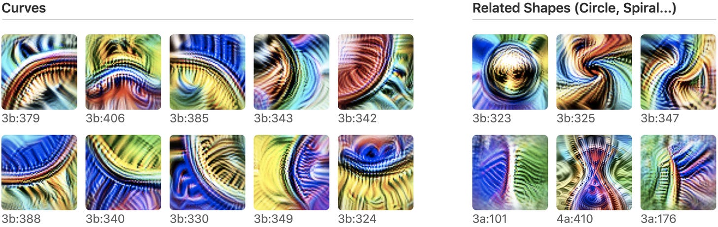
   Image from the "Zoom In: An Introduction to Circuits" post

2. Circuits (computational subgraphs of the neural network) are formed from features connected by weights. These can also be studied and analyzed.
   
   

   

   Image from the "Zoom In: An Introduction to Circuits" post

3. Universality — the most speculative part — similar features and circuits form in different networks solving different tasks.
   

   

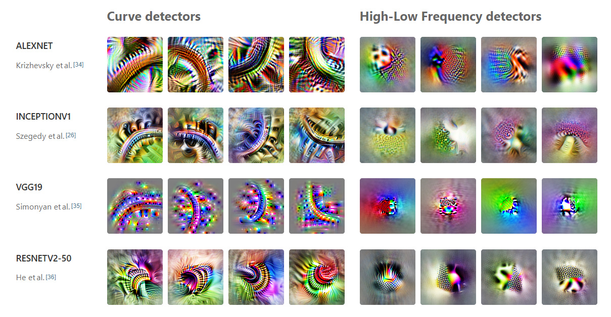
   Image from the "Zoom In: An Introduction to Circuits" post

Well, it's an interesting program. I strongly believe in 1 and 2, though I'm more skeptical about 3, or rather, I believe it with caveats — there should be strong influence from inductive biases and other lower-level things. But it would be interesting if that influence turns out to be not too strong.

This specifically falls into the realm of mechanistic interpretability (mech interp), where we do zoom-in, study learned representations, and search for circuits. I recently wrote a post about the paper on automatic circuit discovery, which presents the ACDC method:

By the way, two big papers were published on this topic last year and this year: “Mechanistic Interpretability for AI Safety -- A Review” and “Open Problems in Mechanistic Interpretability” (this one was just a few days ago).

I also generally prefer related topics, such as developmental interpretability (dev interp), which focuses more on how model structure changes during training, what phases exist, etc. Things like Grokking or the work of the late Naftali Tishby fall more into this category.

Starting with dev interp can be challenging because it likely assumes training. Though if you choose a suitable model object, your own "Drosophila," maybe it's not so difficult... I decided to start with mech interp, where you can already work with pre-trained models, with shorter cycles (otherwise, I’d never finish the course in a reasonable time 🙂).

Along the way, this allows digging into the basics and getting closer to first principles. It feels almost like the good old days of writing in assembly or machine code. It's always good to look under the microscope at what's happening in a transformer at a low level, especially since everyone's gone so high into the clouds nowadays.

Looking Inside Gemma

The prerequisite for the following text is understanding how transformers work, particularly GPT-like models based on the transformer decoder. If you need to build up your understanding in this area, I recommend the excellent visual materials from Jay Alammar:

• The Illustrated Transformer

• The Illustrated GPT-2

• How GPT3 Works

The Gemma 2 2B model

As part of the course, I needed to do a project, and I decided to practically dive into mech interp and dig deeper into the internal representations of the smallest Gemma 2 2B open LLM by Google. Gemma 2 2B is a sufficiently good small model that fits in the memory of an NVIDIA T4 GPU, which I used in Colab.

Gemma's architecture description is in this post or in the original paper.

The ideal goal was to uncover a circuit for a simple task like adding single-digit numbers. However, given the project's short time frame, I’d be happy to look for interesting patterns. Finding circuits probably requires significantly more time, so at least getting a general picture of what happens where inside the network would be valuable.

The whole Colab notebook related to this experiment is here.

I chose Gemma because it has a good tokenizer. In particular, numbers are split into individual digits rather than frequently occurring meaningless digit combinations. This might not be so important for single-digit numbers, but it's useful for future task expansion.

Image from the interesting post on tokenization

Dataset

For starters, I collected several examples of the following form:

At the token level that the model works with, the examples look like this (I limited them to length 9; in reality, they were padded with <pad> tokens to size 32):

The examples are run through the LLM without any additional prompt. You could experiment with prompts, but the base non-instruct Gemma continues the text quite decently with the correct answer and continues generation further, though that part isn't important to me. The output looks like this:

Technically, inside the transformer, there's a prediction of the next token for each position, but we're not interested in any position except the <eos> token — this is where the first token of the answer should appear, and in our case, when the answer is a single-digit number, it's actually the entire answer (though, as we saw, the model won't stop there and will continue generating further). We can work with this, and at least it's clear where to extract the correct (or incorrect) answer.

Code

I used the Keras 3.0 library and keras-nlp to load the model.

The model itself consists of a backbone and an output layer that transforms embeddings into a probability distribution over discrete tokens.

The backbone contains the input layer for transforming token IDs into embeddings, a stack of transformer decoder layers (26 of them from decoder_block_0 to decoder_block_25), and a final RMS normalization layer. The backbone contains the main part of the model's weights, 2,614,341,888 trainable parameters. The token_embedding layer can work in both directions and uses the same set of weights in both the backbone and the main part.

I modified the model to return the final backbone output and the activations of all embedding and decoder layers so they could be analyzed. This is done with relatively simple code:

Activation visualizations

For example, you can visualize embeddings of any layer for given tokens. In the example below (it’s better to look at the notebook), we visualize embeddings for the first nine tokens of our several examples. The embeddings are taken from the last decoder layer before normalization and final output. The left part shows the mean value, while the main part on the right shows the entire multidimensional embedding vector (2304 float32 numbers).

The image is too big for the post; please look at the Colab notebook

We can then analyze how the embedding for the token corresponding to the model's answer is formed.

My expectation was that the embedding of the <eos> token gradually approaches the embedding corresponding to the answer token as it moves toward the network's output. So, in the example "<bos>5+2=<eos>", this embedding should be close to the embedding for the token "7". With the caveat that positional encodings are added to token embeddings, depending on the current position and its surroundings — in Gemma's case, these are RoPE Embeddings, so embeddings of the "7" token in different string positions will be slightly different.

For interest, I compared the last layer embeddings for <eos> token from different examples and the input embedding for the token "7" from the example "2+7=".

Even visually, it's noticeable that the last layer <eos> embeddings differ for different examples, including examples that give the same answer, like "2+5", "5+2", "3+4". If we calculate various similarity measures between this embedding and the embedding of the token "7" from the corresponding example, no interesting pattern is visible. L1, L2, and maximum difference don't show anything interesting, while cosine similarity is below average only for one non-matching example "2+2"and a bit lower than others for the example "2+7". The incorrect example "5-2" gives a value only slightly lower than the correct examples. The choice of threshold here is not obvious. In our toy example, it could be above 0.070, but in reality, everything will likely be much more complex.

As a sanity check when analyzing input embeddings, we can see that they are identical:

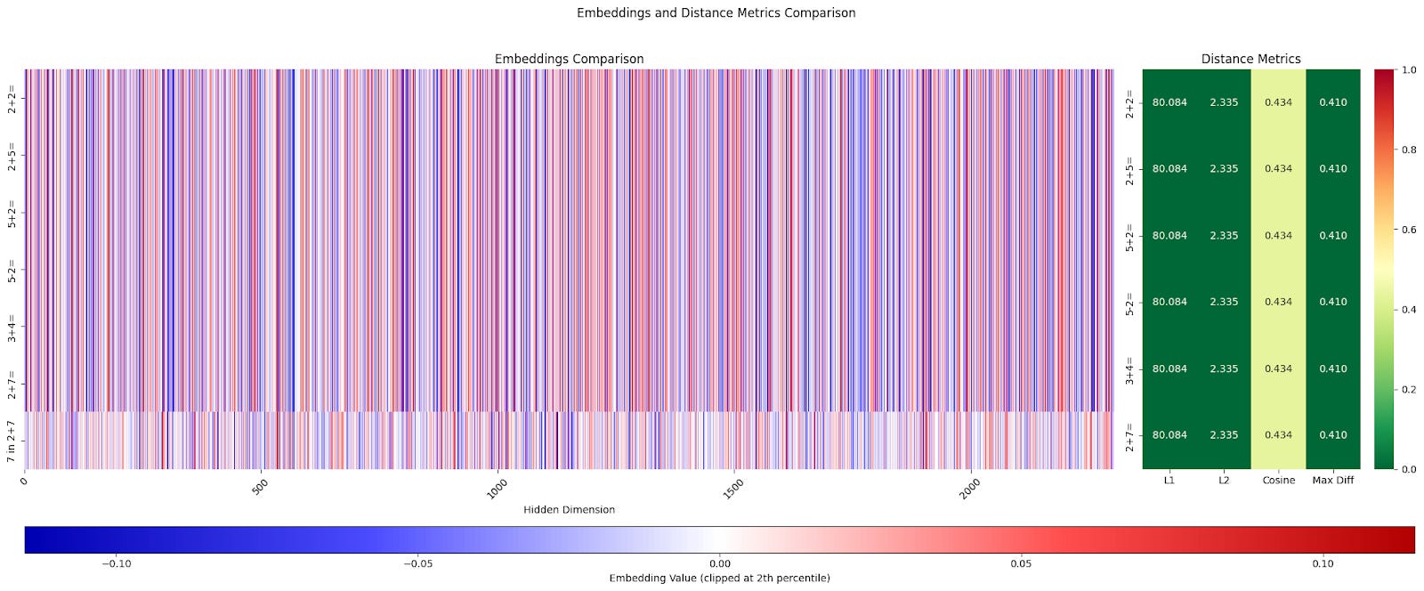
Perhaps a more sophisticated similarity metric or algorithm is needed to determine identical values from embeddings.

Embedding evolution

Either way, as the network operates and information moves from layer to layer, an embedding leading to the correct answer is formed. The evolution of the answer embedding from the model input to the last layer is an interesting visualization:

This was somewhat unexpected for me and turned out to be not as simple as I thought. Something happens in the model at each layer. Even on super simple tasks like "5+2=", all 26 decoder layers do something, and the embeddings change visually.

You can identify separate groups of layers with similar patterns by eye: layers 0-3, 4-12, 13-19, and 20-25. The input (after the embedding layer) and output (after RMSNorm) also stand out.

I previously reviewed a couple of works about creative approaches to layer execution:

I thought the task would be quickly solved inside the model, embeddings would quickly stabilize, and then go unchanged through residual connections to the end so at least some layers won’t be necessary. But this apparently isn't the case.

Analyzing layer importance

At this point, I became interested in whether any significant data transformation occurs in these layers and whether any of the layers could be dropped without losing model performance. In other words, what is the importance of individual layers for obtaining correct results in our model task with single-digit mathematical operations?

You can't collect many examples with just single-digit addition, so I expanded the set of allowed operations to all four basic arithmetic operations and generated a dataset of examples with these operations. Now it includes examples like: '0/7=', '9*0=' '9-2=', '3-0=', '2-1=', '2+1=', '4+5=', '7-4=', '0/5=', '1+2=', etc. I generated a dataset of 1000 examples to get any statistically significant results.

For the experiment, I wrote code that removes specified layers from the model's backbone or instead assembles a new backbone from only the listed layers (see the Colab notebook). This is somewhat similar to the ACDC circuit search method, which also tries to remove elements from the network while maintaining result quality. In ACDC, the elements are computational graph edges; in our approach, they are entire network layers.

I limited myself to configurations with a single missing layer and generated 26 backbones where one of the existing layers is absent, sequentially going through layers from first to last.

For each backbone configuration, all 1000 examples are computed, and their results are checked. As output, we have an indicator of 0 or 1 for each example showing whether the computation was correct. We also calculate the accuracy of this configuration, showing the proportion of correct answers.

The graph below shows the task solution accuracy depending on which layer was removed from the model:

Here the result was also unexpected for me, as clearly more important layers for this task are visible.

The first decoder layer (index 0) turned out to be very important. This could be expected since processing starts immediately, and some important primary stages probably happen here. If these are skipped, the network can't do anything further since it relies on them.

More unexpected was the high importance of layer #4. Visually, in the embedding evolution picture, this layer also stands out from others with a seemingly different pattern with visibly lower activation magnitudes. From it until layer #10, there's some weakly expressed but stable activation pattern with relatively low magnitudes. The accuracy graph shows that each subsequent layer after the fourth affects the result less and less.

Then roughly from layer 13 to 19, another pattern with higher magnitudes is noticeable, and the accuracy graph also shows a relative quality drop in this area.

Layers 22 and 23 affect accuracy the least, while the last two layers, 24 and 25, are slightly more important.

This suggests that within the decoder stack, groups of layers form some structure and implement different functions that affect result quality differently.

All this requires further deeper investigation. Perhaps this is all an artifact of this specific model or specific task and dataset. But maybe not. The result is interesting and unexpected for me, even though I've really just scratched the surface.

Next Steps

For those wanting to verify and continue my research, I've made the Colab notebook code available: https://colab.research.google.com/drive/1Dita8PWjxc_nPjOKCGKyuv7tVamZIc-h?usp=sharing

Here are the next steps that I think are worth trying:

1. Other Tasks

   1. Test the model on more complex tasks of the same nature, for example, operations with two-digit and three-digit numbers

   2. Test the model on a somewhat different task, for example, Boolean logic

   3. Test the model on a set of very different tasks: question answering, linguistic tasks like part of speech tagging, etc.

2. Other Models

   1. Test on other models of the same family: Gemma 2 2B Instruct, Gemma 7B

   2. Test on models from other families: Llama 3.2 (1B, 3B), Qwen, etc.

   3. Particularly interesting to test on a model with a different architecture: RecurrentGemma

   4. Test on distilled models to check if the pattern is preserved during distillation. For example, DeepSeek-R1 and DeepSeek-R1-Distill-Qwen/DeepSeek-R1-Distill-Llama might be interesting choices.

3. If patterns reproduce, it would be interesting to understand layer specialization in more detail.