Tiny Recursive Model

Less is More: Recursive Reasoning with Tiny Networks

Authors: Alexia Jolicoeur-Martineau
Paper: https://arxiv.org/abs/2510.04871
Code: https://github.com/SamsungSAILMontreal/TinyRecursiveModels

The recently discussed HRM (Hierarchical Reasoning Model) demonstrated an interesting result with a small model size, but subsequent analysis from the ARC-AGI organizers showed that the result is primarily influenced by sequential answer improvement (deep supervision), while recursion in the H and L modules doesn’t add very much.

The new work on TRM (Tiny Recursive Model) questions the necessity of all this complexity and follows the philosophy of “less is more.” The new TRM model contains 5M-19M parameters (there are nuances), versus 27M in HRM.

Both the paper and this breakdown make sense to read after you’ve already read about HRM, because the entire paper is structured as a systematic analysis of HRM.

Also, it’s important to constantly remember that comparing HRM/TRM with traditional LLMs is in many ways flawed — these are models of completely different classes. LLMs are quite general models trained on the entire internet on text continuation tasks, including complex finetuning for chat, instructions, solving various problems in mathematics and other disciplines, etc. The fact that they’re also capable of solving sudoku, mazes, and ARC-AGI tests is actually quite surprising to me. All modern LLMs are transformer-decoders (there are hybrids with SSM, but that’s not important here). HRM/TRM are transformer-encoders (like BERT); they don’t continue any sequence token by token, they process all tokens at once and generate a new sequence of the same length as the input. HRM/TRM (unlike BERT, which was also trained on roughly the entire internet) are trained only on one specific task from a list; there’s no talk of any universality here yet. So all those enthusiastic posts saying that a model a million times smaller has appeared and is beating the best top LLMs and soon they’ll all be done for, data centers aren’t needed, etc. — you need to divide by that same million; many of the authors haven’t really understood what was done.

🩼 What Was Wrong with HRM

There were several aspects in HRM that potentially required improvement:

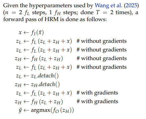
• Implicit Function Theorem (IFT) with 1-step gradient approximation: There’s a question about backprop only through two of all the recursions (the last state of H and L), which I also wondered about. There’s no certainty that IFT is applicable to this case with HRM. It’s not even certain that a fixed point is achieved. The original work’s authors used two recursion steps at each level (H and L), and it turns out that HRM assumed achieving a fixed point by both modules only after two forward passes of L, one H, and again one L. This raises doubts.

  

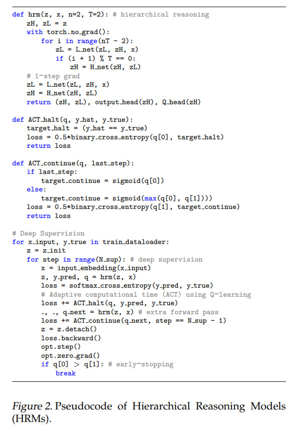
• ACT (Adaptive Computation Time): reduced the amount of computation but had its own cost. Q-learning for continue/stop values required an additional forward pass through HRM.

• References to biology: The authors created HRM initially with reference to biological processes and (correlationally) confirmed the analogy with the real mammalian brain. This is interesting but doesn’t explain why HRM was made exactly as it was made.

• No ablations were done: and without them, it’s unclear how much the biological arguments and the fixed point theorem actually matter, and which of HRM’s components are important and why. Why two latent features and not some other number is also unclear.

The idea of the TRM authors is that you can simplify HRM and the recursive process in it, and understand the model without needing biological arguments, fixed point theorems, hierarchical interpretations, and two different networks. At the same time, they explain why 2 is the optimal number of features (z_L and z_H).

🏗 TRM Architecture

The model is designed so that there’s one small network, which is essentially a standard transformer block: [self-attention, norm, MLP, norm]. In the original idea, there were 4 such blocks (but after experiments they came to 2).

At the input, it has three elements: input (x), latent (z), and prediction (y); they’re all summed into one value. At the very beginning, only x arrives, everything else is zeros (?). The basic iteration, analogous to the L module in HRM, generates a latent value (z, also denoted in the recursion formula as z_L) at the layer output, and the updated z goes back to the module input, where it now adds to input (x) not as zero. The output-prediction (y, also denoted in the formula as z_H) is also added, but since it hasn’t been updated, it doesn’t change anything. The value z_H will only be calculated at the end of the iteration based on z_L and the previous z_H; input x doesn’t participate here.

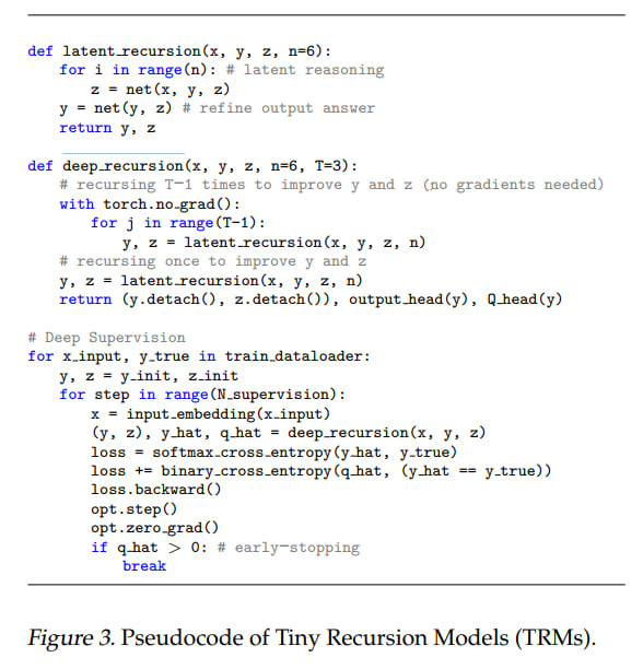
Training essentially happens at three levels. The process described above is the deepest level, called latent_recursion(). In total, TRM’s recursive process contains n computations of f_L and one computation of f_H, backprop goes through the entire recursion, there’s no longer a need to rely on fixed point theorems.

One level up, you can also run several iterations of f_H, sequentially improving both values z_L (z) and z_H (y). This process is called deep_recursion().

Finally, one more level up, besides the recursive process, there’s also deep_supervision (not present as a separate function), like in HRM. The training loop includes up to Nₛᵤₚ=16 supervision steps. At each step, the model performs the deep recursion process:

1. Inner loop (latent recursion): First, the network updates the hidden reasoning feature z for n=6 steps (z ← net(x, y, z)), then refines the answer y once (y ← net(y, z)).

2. Outer loop (deep recursion): The inner loop runs T=3 times. The first T-1=2 executions run without gradient tracking to efficiently approximate hidden states to a good solution. The last execution allows gradients to pass through all n+1=7 network calls. The resulting (y,z) are then detached from the computation graph and used to initialize the next supervision step.

This structure allows a tiny two-layer network to achieve an effective depth of 42 layers at each supervision step (as I understand it, this is (6+1) inner loop steps * 3 outer cycles * 2 layers), which can ultimately significantly exceed the 384 layers that its predecessor HRM achieved (here it would be 42*16=672 layers).

🤔 Reinterpreting HRM

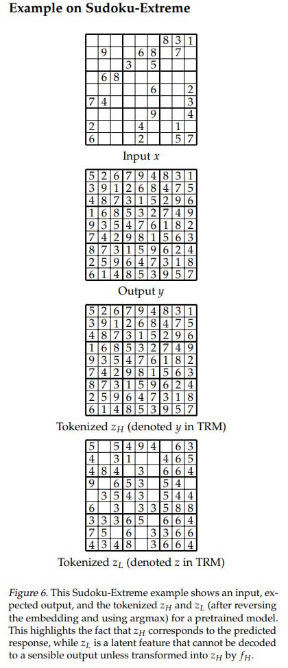
This generally ideologically repeats HRM’s hierarchical approach with two networks/features/latents. Here you can ask the question: why two hierarchical features, not one, not three or some other number? The authors offer their own explanation, reinterpreting the z_H feature as an embedding of the current solution, which if necessary will be converted to an output token through the network’s output head and argmax. The z_L feature, in turn, is a latent feature not directly related to the output solution, but which can be transformed into it through f_H. In such an interpretation, hierarchy isn’t needed: there’s input x, there’s a proposed solution y (formerly called z_H), there’s a latent feature for reasoning z (formerly z_L). The model sequentially improves its latent z, and then based on it and the previous solution y, produces a new y (but can stay with the old one if it’s good).

In total, TRM offers a much simpler and more intuitive interpretation:

• y (formerly z_H): Current (in embedding form) output answer.

• z (formerly z_L): Hidden feature representing the reasoning trace or “chain-of-thought.”

This doesn’t affect the algorithm itself; it’s just a reinterpretation for better understanding, and it’s an answer to why there are two features: keeping in memory the context of question x, previous reasoning z, and previous answer y helps the model iterate its solution, next reasoning z, and next answer y. If you don’t pass the previous z, the model won’t know how it arrived at the previous solution. If you don’t pass the previous y, the model won’t know what the solution was before and will be forced to store it somewhere inside z instead of using z for latent reasoning.

Interestingly, this differs from latent reasoning in the Coconut style; there it was at the token level during autoregressive generation, while here it’s more at the level of model call depth; the unrolling happens in a different dimension.

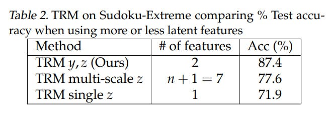
The authors tried different numbers of features, both larger and smaller. One variant split z into multiple features z_i, and each recursion iteration updated one specific feature from them, carrying all others as is. Quality dropped relative to the two-feature variant (but I wouldn’t be surprised if the next work finds reasons for this, like problems with gradient signal, and proposes hacks to make it work). The authors explain this by saying there’s no reason to split z into multiple parts. The other extreme, with one feature z_H, led to an even more serious drop in quality. The authors explain this by the model’s need to store solution y inside z (but maybe you just need to scale the hidden embedding?).

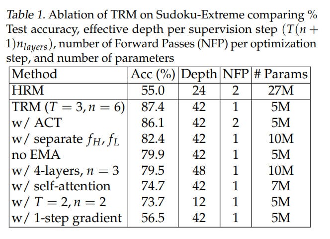
In the proposed scheme, the need for two separate networks H and L (and accordingly for 2x parameters) also disappears — the task being solved z ← f_L(x + y + z) or y ← f_H(y + z) is determined by the presence or absence of x at the input (but what this means at the level of model training and embedding structure is a question for me). As a result, we have one network instead of two, and ablations showed this gives an improvement on Sudoku-Extreme from 82.4% to 87.4% (but again, I wouldn’t be surprised if with scaling it turns out this actually matters; they just undertrained and didn’t throw in as much compute as needed).

🗼 Other Architectural Modifications

The authors tried adding more layers to the model but got overfitting. As they write, “Surprisingly, we found that adding layers decreased generalization due to overfitting.” I don’t know, honestly, what’s so surprising here — ML 101 stuff, but whatever. In the modern age, apparently everyone’s used to the idea that you need to scale.

In the other direction, reducing layers but increasing the number of recursions so that effective depth and compute amount remain the same, they found that 2 layers is optimal, giving an improvement on Sudoku-Extreme from 79.5% to 87.4%, and the number of parameters is half (5M instead of 10M). The authors reference the work “Fixed Point Diffusion Models” (https://arxiv.org/abs/2401.08741), where two layers also seemed optimal in the context of deep equilibrium diffusion models, but there performance was similar to heavier models, while here it’s actually higher. Less is more. A small network combined with deep recursion and deep supervision allows bypassing overfitting with a small amount of data. It would be interesting how it would be with dataset scaling.

There was an experiment influenced by MLP-Mixer (https://arxiv.org/abs/2105.01601) with replacing self-attention with MLP operating on the entire sequence length, since it requires fewer parameters for the case when context length (L) is less than hidden dimensionality (D). This improved the result on Sudoku-Extreme from 74.7% to 87.4%, but worsened for Maze-Hard and ARC-AGI, which require larger context.

TRM simplifies the adaptive computation time (ACT) mechanism. You can abandon the separate computation for continue loss; it’s sufficient to have halting probability, then minus one forward pass of the model, but still sufficiently accurate determination of when the model needs to stop, which significantly speeds up the process. This gave a weak improvement from 86.1% to 87.4% (it’s unclear what the confidence intervals are here).

They also implemented exponential moving average (EMA, 0.999) for weights, since with a small amount of data, the model quickly overfits and starts to diverge; this also improves quality from 79.9% to 87.4% (or rather worsens from 87.4% to 79.9% when removed from the full model). As I understand it, the previous smoothed value of model parameters is taken with weight 0.999 and the new one is added with weight 0.001.

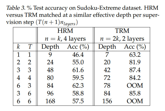
They tuned the number of recursions, found optimal values for HRM T = 3, n = 3 (equivalent to 48 recursions) and for TRM T = 3, n = 6 (42 recursions), this is on Sudoku-Extreme. TRM requires backprop through the entire recursion depth (though T doesn’t affect this; remember, there T-1 steps are done without gradient), so increasing starts to lead to Out of Memory.

🧪 Experiments

Testing is the same as in the HRM paper: ARC-AGI-1 and -2, Sudoku-Extreme, Maze-Hard.

In Sudoku-Extreme, 1K examples were used for training and validation on 423K examples. Maze-Hard has 1000 examples each in training and test. So it seems like in HRM, maybe with adjustments for random seed and specific sampling of the thousand examples. For ARC-AGI, the ConceptARC dataset was also used for augmentation (this doesn’t seem to be like in HRM, but similar to what the ARC-AGI team did in their verification). I’m also not sure about augmentations — whether they completely repeated those from the HRM paper; you’d need to dig deeper. The numbers for HRM are exactly the same as in the original paper, so they probably took them from the paper itself, but on the other hand, the code for HRM is also in the TRM repo.

Overall result: TRM achieves even higher numbers than HRM:

• 74.7%/87.4% (attention version/MLP version) versus 55% for Sudoku

• 85.3% (attention version, MLP version gives 0) versus 74.5% for Maze

• 44.6%/29.6% (attn/MLP) versus 40.3% for ARC-AGI-1

• 7.8%/2.4% (attn/MLP) versus 5.0% for ARC-AGI-2

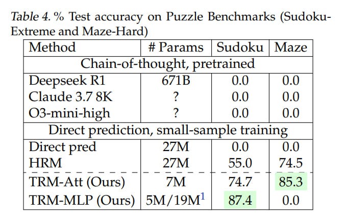
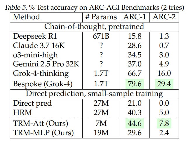
Interestingly, for sudoku the MLP version works better; for others requiring larger context, the attention version is better. The TRM version with attention contained 7M parameters, the MLP version — 5M for Sudoku and 19M for other tasks. HRM was always 27M.

The appendix has a small section on ideas that didn’t work. Among them:

• Replacing SwiGLU MLP with SwiGLU MoE — generalization dropped significantly, but possibly with more data it would be different.

• They tried passing gradients through less than the entire recursion — for example, only through the last 4 steps — didn’t help at all, only complicated everything.

• Removing ACT made everything worse

• Shared weights for input and output embeddings made everything worse

• Replacing recursion with fixed-point iteration from TorchDEQ slowed down and worsened things. Possibly this is additional confirmation that convergence to a fixed point isn’t important.

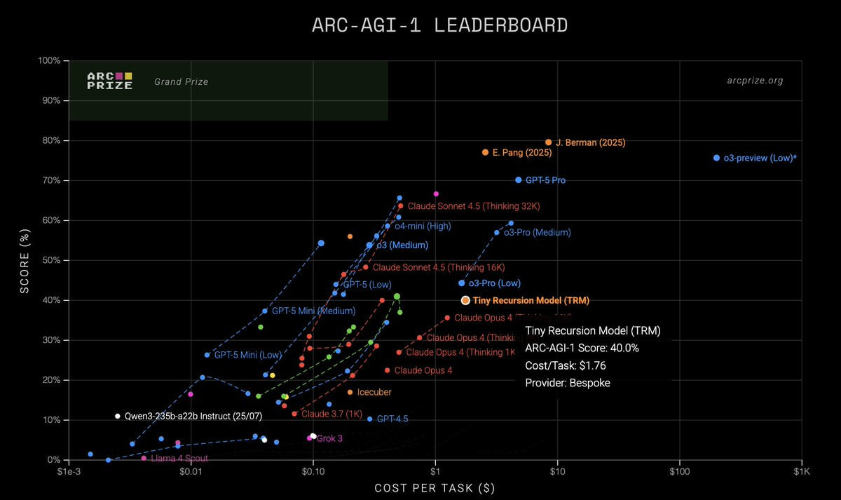
ARC-AGI verified the results for TRM:

• ARC-AGI-1: 40%, $1.76/task

• ARC-AGI-2: 6.2%, $2.10/task

Here the variance between the paper and ARC’s own measurements is smaller than it was for HRM.

TRM is smaller, but runtime consumes more (unsurprising with recursion present). Perhaps the better results aren’t because the model is smarter, but because it trained longer? I didn’t understand how equal the models are in terms of spent FLOPS; it would be interesting to look at.

---

In short, the work is cool, the empirical result is interesting. There’s no feeling that the theoretical part is deeply understood — why exactly these recursions work so well. Also, this work is a cool example of some architectural inventiveness as opposed to eternal model scaling (though scaling this specific one is also interesting, as is extending it to other classes of tasks). I think there will be developments. The experiments don’t look very expensive; runtime from <24 hours to about three days maximum on 4*H100 according to the repo.

Good recursions to everyone!