Hierarchical Reasoning Model

Authors: Guan Wang, Jin Li, Yuhao Sun, Xing Chen, Changling Liu, Yue Wu, Meng Lu, Sen Song, Yasin Abbasi Yadkori
Paper: https://arxiv.org/abs/2506.21734
Code: https://github.com/sapientinc/HRM

A hierarchical longread for your weekend!

I didn’t get around to doing a manual breakdown of this HRM work from the Singaporeans at Sapient Intelligence back in the day (though I did do an automatic one), but it’s important and worth breaking down. Especially since the recent TRM was inspired by it.

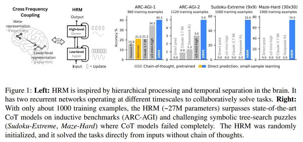
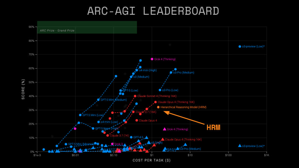
This interesting summer work proposed a brain-inspired hierarchical model with fast and slow networks. The model was quite modest in size (27M) and was trained on only 1000 examples. Yet it achieved very high scores on several challenging tasks. In particular, it also managed to beat o3-mini-high (as well as the giant DeepSeek-R1 and Claude 3.7) on ARC-AGI-1 and 2, which is pretty cool. What’s behind this model and how does it work? Let’s break it down.

Modern transformers have achieved significant results across various tasks, but their architecture itself is generally quite shallow with fixed depth (though there are exceptions with recursion or dynamic depth). Because of this, they’re limited to low computational complexity classes (such as AC⁰ or TC⁰) with fixed-depth circuits and struggle with problems requiring deep, iterative, and algorithmic reasoning. Let me remind you that RNNs sit in a higher class and are generally Turing complete. More details on complexity classes here.

Inspired by the hierarchical processing at different temporal scales inherent in the human brain, the authors present the Hierarchical Reasoning Model (HRM) — a new recurrent architecture.

🏗 HRM Structure

At the core of HRM lie three principles observed in neural computation: hierarchical processing, temporal separation, and recurrent connections. The architecture includes two interdependent recurrent modules operating at different temporal scales:

1. A high-level (H) module for slow, abstract, and deliberate planning.

2. A low-level (L) module for fast, detailed, and subordinate computations.

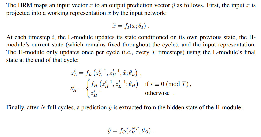
The model’s dynamics unfold over N high-level cycles, each consisting of T low-level time steps. The L-module updates at each step, and its state depends on the H-module, which remains unchanged throughout the entire cycle. The H-module updates only once per cycle, using the final state of the L-module.

- Hierarchical Convergence

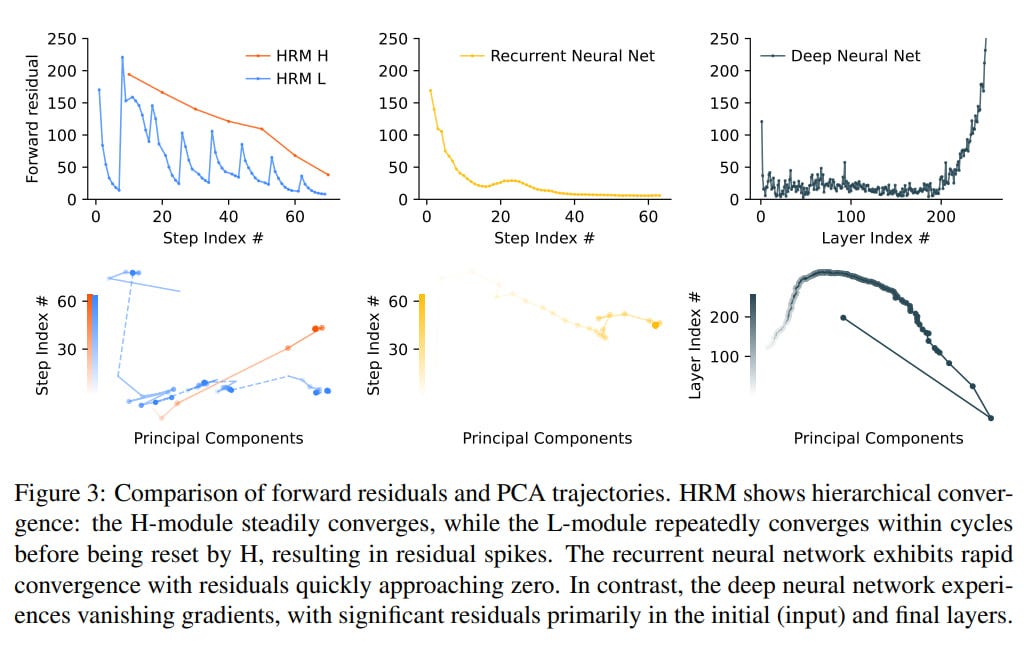
Standard RNNs tend to converge prematurely. When the hidden state settles near a fixed point, the magnitudes of updates decrease, effectively freezing subsequent computations and limiting the network’s effective depth. We want convergence to be gradual, but engineering this approach is difficult. HRM combats premature convergence through a process the authors call hierarchical convergence. In each cycle, the L-module converges to a local equilibrium, but it depends on the high-level state that the H-module provided for that cycle. After T steps, the H-module incorporates the resulting output and updates its state, thereby setting a new context for the next L-module cycle, which will now converge to a different local equilibrium.

This is like a project manager (H-module) who sets a specific subtask (for example, “solve this corner in sudoku”). The L-module acts as an executor who rapidly iterates to solve this specific subtask. Once the executor finishes, they report back, and the manager uses this result to set the next subtask. This prevents the model from getting stuck and allows it to perform structured, multi-step computations, maintaining high activity throughout many steps and achieving an effective depth of NT.

- Approximate Gradient

A key innovation of HRM is its ability to efficiently train such deep recurrent processes. The model sidesteps memory-intensive and biologically implausible Backpropagation Through Time (BPTT), which requires O(T) memory. Instead, it uses a one-step gradient approximation, theoretically grounded in Deep Equilibrium Models (DEQ).

This approach uses the Implicit Function Theorem (IFT), which allows computing the gradient of a fixed point without unrolling the computation. By approximating the inverse Jacobian matrix (I - J_F)⁻¹ with the identity matrix I, the model can compute gradients with constant memory consumption O(1). Essentially, this simplification assumes that each recurrent step is a stable refinement, allowing the model to compute the gradient by backpropagating only through the most recent computational step, rather than unrolling the entire history.

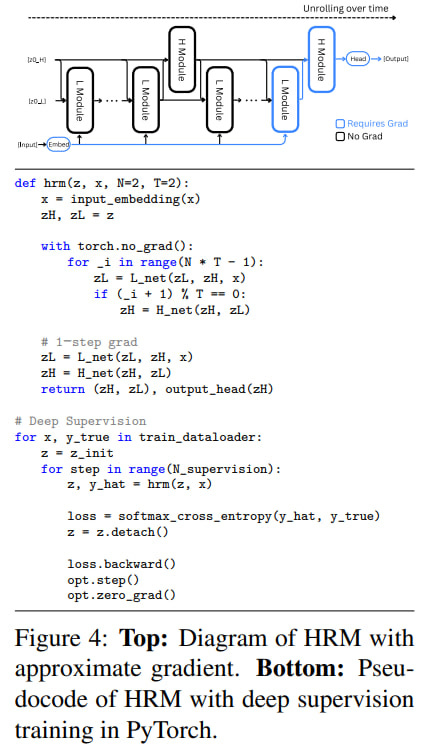
As a result, the gradient from output to input flows through the final state of the H-module to the final state of the L-module and then to the input. At first glance, it seems we lose a lot by not passing the gradient through all final L states and their corresponding H states, but maybe in the next version.

- Deep Supervision

To further stabilize training, HRM uses deep supervision, inspired by the principle that neural oscillations regulate learning in the brain. Maybe I didn’t fully understand the idea, but it seems to me that the very presence of H and L modules is already a direct reference to dynamics unfolding at different frequencies, with all these alpha, beta, theta rhythms. But on the other hand, this supervision can be viewed as an implicit module at an even higher level than H; I’d call it S.

For each sample (x,y), multiple forward passes of HRM are performed, each called a segment. At the end of each, the loss is calculated and parameters are updated. Importantly, the hidden state is detached from the computational graph before being passed to the next segment, which acts simultaneously as a regularizer and an effective training signal. That is, gradients from segment m+1 don’t affect segment m. This strongly resembles the recycling approach in AlphaFold 2, where the 3D protein structure from the system’s output was sent back to the input for subsequent refinement.

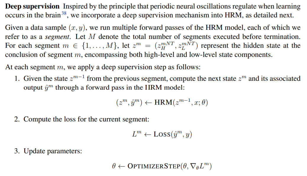
The number of segments is determined dynamically through ACT.

- Adaptive Computational Time (ACT)

This is actually my favorite topic; I’ve written about ACT extensively before.

Inspired by the brain’s ability to switch between fast, automatic thinking (”System 1”) and slow, deliberate thinking (”System 2”), HRM integrates ACT. A Q-learning algorithm decides to “stop” or “continue” computations after each segment, based on the H-module’s state.

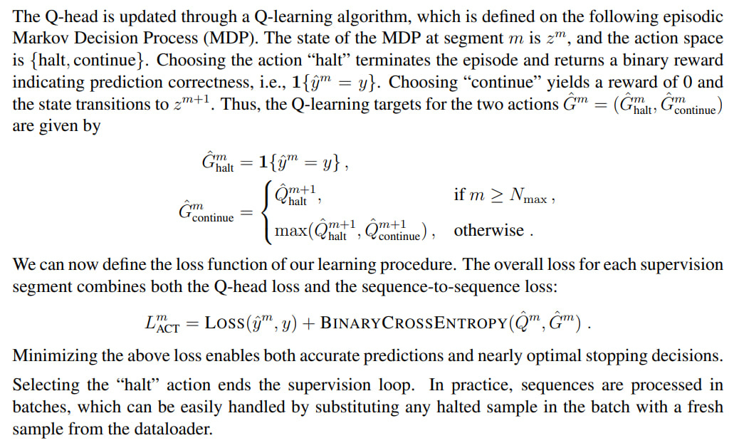
The number of segments is capped at M_max (hyperparameter) with probability ε and floored at M_min (a random variable obtained by uniform sampling from the set {2, …, M_max}), and with probability 1−ε is set to 1. Stopping occurs when we exceed M_max or when the Q-value for stopping (Q_halt) exceeds Q for continuing (Q_continue) and we’ve already exceeded M_min.

The overall loss function combines the standard loss for the sequence-to-sequence task with Q-learning loss, allowing the model to dynamically allocate computational resources. Overall, the ACT process allows achieving quality comparable to a fixed run of M_max segments while spending significantly fewer computational resources.

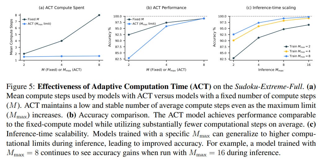
For inference-time scaling, it’s sufficient to set M_max higher without any additional training.

Another recent example of using ACT in recursion is the Mixture-of-Recursions (MoR) work.

- Implementation

Both modules, H and L, are implemented using modern transformer-encoder blocks (hello, BERT!), incorporating improvements such as Rotary Positional Encoding (RoPE), Gated Linear Units (GLU) by Noam Shazeer, and RMSNorm in a Post-Norm architecture. Input and output are token sequences of length l.

The modules are combined through simple element-wise addition, which is easy since their architectures are identical. In the future, they plan more sophisticated combinations, for example, with gating.

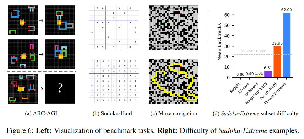
The model is not an LLM trained on the entire internet (moreover, it’s not a decoder at all, but an encoder), and is trained on specific tasks: ARC-AGI-1 and -2, Sudoku-Extreme 9x9 with particularly difficult puzzles (3.8M total, of which 1000 were selected for training), Maze-Hard 30x30 (also 1000 each in train and test).

📊 Results

The experimental results are impressive. Trained from scratch on only ~1000 examples per task and having just 27M parameters, HRM demonstrates very high performance where much larger models fail.

For ARC-AGI, there were many augmentations with rotations, shifts, etc. of test examples. For sudoku, many permutations. For mazes, nothing was done.

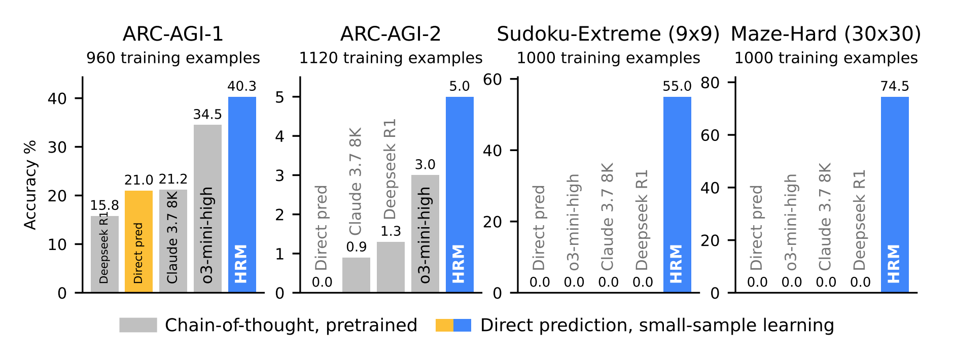
In complex symbolic tasks such as Sudoku-Extreme and Maze-Hard, which require extensive search and backtracking, HRM achieves high accuracy of 55% and 74.5%. Meanwhile, state-of-the-art CoT models completely fail, scoring 0%, as does Direct pred — replacing HRM with a transformer of similar size with 8 layers trained on similar data.

On the ARC-AGI-1 benchmark, a test of general fluid intelligence, HRM achieves 40.3% accuracy, significantly surpassing larger CoT models such as o3-mini-high (34.5%) and Claude 3.7 (21.2%), as well as Direct pred at 21%. On ARC-AGI-2, a proud 5%, but o3-mini-high only has 3%, others even less, and Direct Pred 0%.

Experiments with training on the full sudoku dataset (which is 3.8M) show that first, increasing depth is important and scaling transformer depth with fixed width leads to noticeable improvement, while increasing width with fixed depth doesn’t help at all.

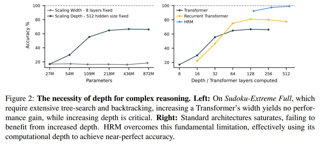
Second, while the performance of standard as well as recurrent (didn’t understand implementation details) transformers plateaus with increasing depth, HRM effectively uses its recurrent depth to solve complex problems and achieves nearly 100%. Though for HRM only three points are given; it would be interesting to see how it would behave at the beginning of the graph.

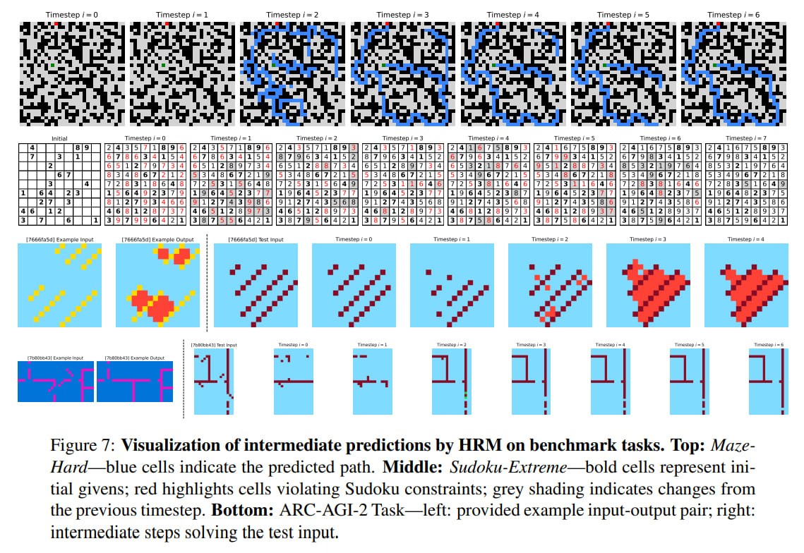
Visualizations of the model’s intermediate steps show adaptive reasoning strategies. For the maze, this is parallel exploration of multiple paths and elimination of blocked or inefficient ones, then creation of a preliminary version and its refinement. In sudoku, it resembles depth-first search with backtracking. For ARC tasks, it’s incremental additions to the board and iterative improvement without backtracking, resembling hill climbing. So it learns different strategies for different tasks, and I suppose it is similar to AlphaZero, the system capable of learning several games.

🤯 Emergent Brain-Like Structure

An interesting section of the paper is called Brain Correspondence. Perhaps the deepest finding is the emergence in the trained model of a neuroscientifically plausible structure, serving as validation of its core design principles. The authors were inspired by brain function (hierarchical processing at different temporal scales), and remarkably, the trained model spontaneously developed a key feature of the brain’s physical structure (hierarchy of representation dimensionality). The authors analyzed the effective dimensionality of the hidden states of the H- and L-modules using the Participation Ratio (PR) and obtained the following results (Fig 8 c,d):

• The high-level (H) module develops a high-dimensional, high-capacity representation (PR ≈ 89.95) that scales with task diversity.

• The low-level (L) module maintains a stable, low-dimensional representation (PR ≈ 30.22).

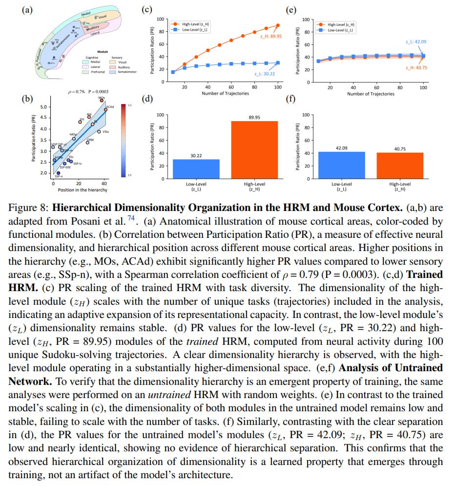
This emergent hierarchy, absent in the untrained network (Fig 8 e,f), precisely mirrors the dimensionality organization observed in mammalian cortex (Fig 8 a,b), where higher-order associative areas have higher dimensionality than primary sensory areas. This provides correlational evidence that HRM learns a fundamental organizational principle for flexible general-purpose reasoning.

🧠 Post-Analysis from ARC-AGI

The ARC competition organizers analyzed HRM’s performance and tested it on the hidden part of their dataset. They confirmed the model’s results; on Semi-Private sets it’s 32% for ARC-AGI-1 (which is still cool for such a small model) and 2% on ARC-AGI-2.

The most interesting part is in the ablations performed. They are as follows:

• Hierarchy with recursion doesn’t really matter; a transformer of the same size with all other architectural factors unchanged (but HRM does consume more compute, which may have an effect) gives quality in the range of +/-5%, especially if doing only one cycle (segment). So it’s not about the architecture per se. This isn’t entirely clear — why did Direct pred then have a 2x difference?

  

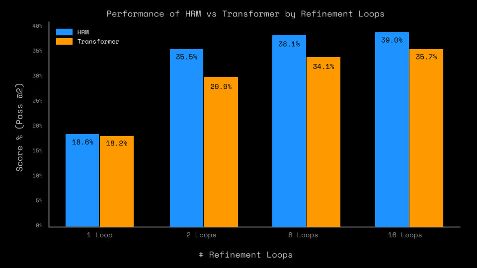
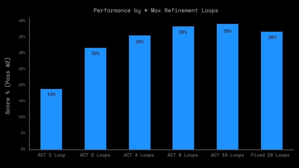
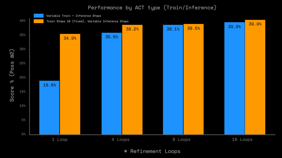
• The outer-loop refinement process (that same Deep supervision with ACT and sequential result improvement) adds a lot, especially at training time. The biggest difference is between one and two passes, but overall quality continues to grow up to 16 cycles. So Universal Transformer or ALBERT — that’s our everything?

  

  

• Cross-task transfer is limited; most of the performance comes from memorizing solutions to specific tasks.

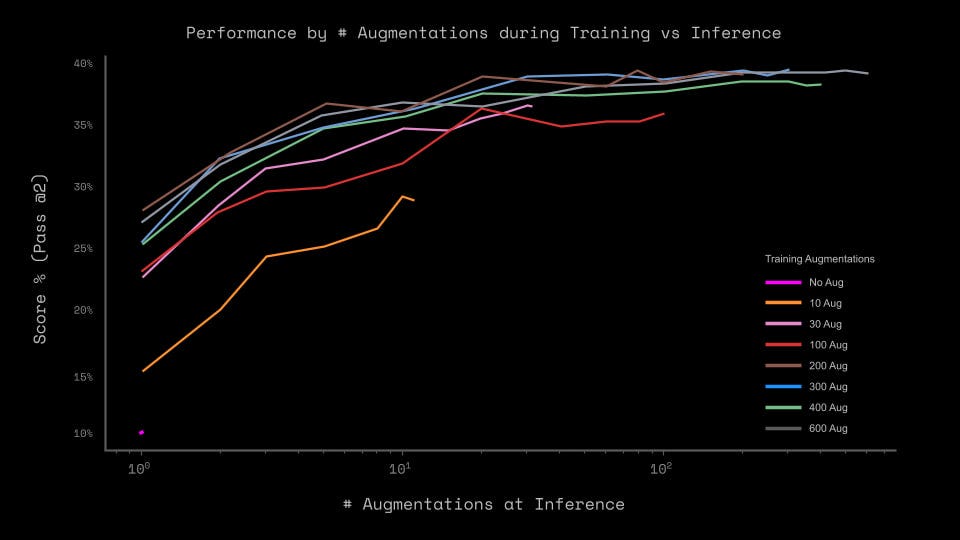
• Augmentations in pretraining are critical, but 300 are sufficient, not 1000. Augmentations at inference add little.

  

The analysis authors say this makes the approach fundamentally close to that presented in the article “Arc-agi without pretraining”, but the HRM paper states that the mentioned approach gives as much as the Direct Pred baseline. So maybe fundamentally close, but the quality difference is almost twofold.

🤔 Limitations and Future

The authors acknowledge several limitations. The one-step gradient is an approximation, and evidence for the causal role of the emergent dimensionality hierarchy is still correlational. The connection between modules is implemented as simple element-wise addition, which could be improved with more sophisticated gating mechanisms. Future work includes investigating the causal necessity of the emergent hierarchy and integrating hierarchical memory for processing even longer contexts.

💀 Historical Context

HRM’s ideas have deep roots, and it’s worth looking at predecessors to understand that this is good old ideas well forgotten.

- Neural History Compressor (Schmidhuber, 1991-1992)

Back in the early 90s, Jürgen Schmidhuber proposed the Neural History Compressor — a hierarchy of recurrent networks trained to predict their inputs at multiple self-organizing temporal scales. The key idea: each RNN in the stack learns to predict its next input, and only unexpected inputs (prediction errors) are passed to the next, higher level, which operates more slowly. Information is compressed but not lost — it simply transitions to a different temporal scale. The mechanism is surprisingly similar to hierarchical convergence in HRM: the low level works fast and processes details, the high level works slowly and manages overall strategy. Schmidhuber even proposed a “collapsed” version with two networks — chunker (high level) and automatizer (low level) — just like the H and L modules in HRM.

- Clockwork RNN (Koutník et al., 2014)

20+ years later, the team of Koutník, Greff, Gomez, and Schmidhuber presented Clockwork RNN — a more practical implementation of the multi-scale idea. The hidden layer is divided into modules, each processing inputs at its own “clock frequency” — some update every step, others every 2, 4, 8 steps, etc. This creates a natural separation into fast and slow processes.

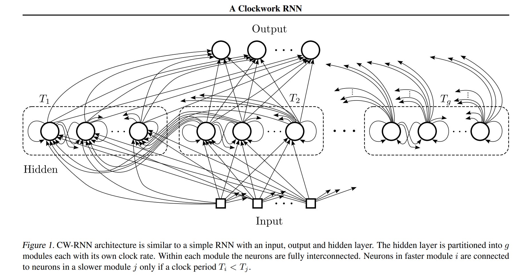
HRM explicitly references Clockwork RNN and is its logical continuation, but with important improvements: (1) not fixed frequencies but adaptive convergence, (2) modern transformer blocks instead of simple RNNs, (3) efficient training without BPTT through the DEQ approach.

- Fast Weights (Hinton, 1987/2016)

Geoffrey Hinton proposed the concept of “fast weights” back in 1987, then returned to it in 2016 with Ba et al.. The idea: each connection has two weight components — slow (long-term memory, learns and decays slowly) and fast (short-term memory, learns and decays quickly). This allows efficiently storing temporary memory of the recent past without copying activation patterns.

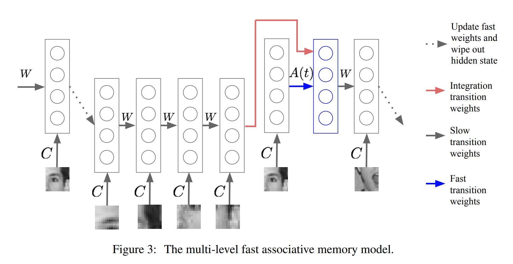
Although technically implemented differently (in HRM the separation is at the module level, not weights), conceptually it’s very close: fast processes for short-term context, slow ones for long-term planning. Moreover, Hinton explicitly motivated this with biology — synapses have dynamics at different temporal scales.

- Other Related Work

• Hierarchical Sequential Models (Hihi & Bengio, 1996) — an early attempt to capture long-range dependencies through hierarchy

  

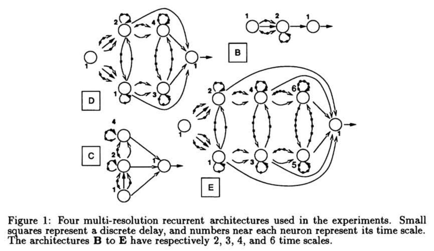
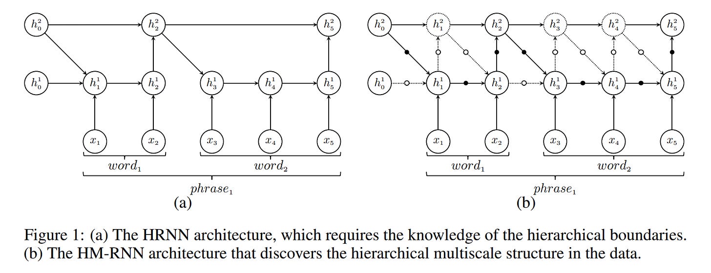
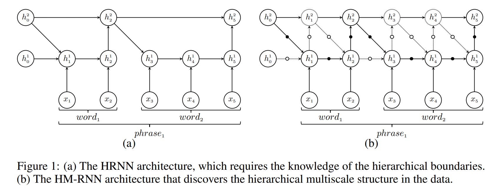
• Hierarchical Multiscale RNN (Chung et al., 2016) — later work where slow LSTM receives inputs less frequently

  

• there could be many other works here

It’s interesting that ideas of hierarchical RNN with different temporal scales appeared again and again over 30+ years, but only now, with the right combination of techniques, are they showing impressive results. Perhaps the time for these architectures has finally come.

---

Cool work, in short. It has already influenced another recent buzzworthy work “Less is More: Recursive Reasoning with Tiny Networks” about Tiny Recursive Model (TRM). I’m planning to break that one down next.